I received a comment from a reader recently on my post, Display of SSAS KPI Indicators in Excel, which asked:
Would it be possible to use the status to configure "conditional formatting" on the value column?
To which the response is, absolutely! Here’s how I set it up in a simple spreadsheet, created from the Adventure Works 2008 cube project:
Let’s say our business rule is: Give the Revenue column a back color of yellow if the Status is not satisfactory.
Formula to Format Cells
1. Select cell B4, which is our first Actual value.
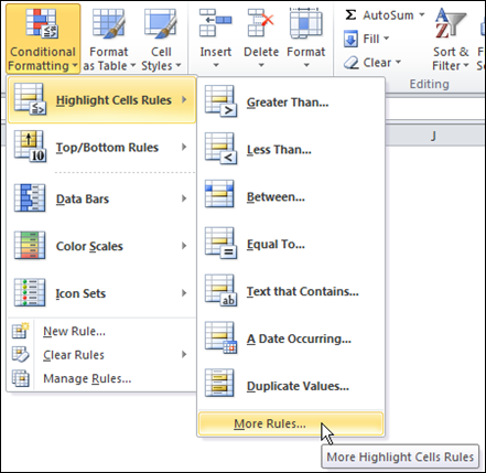
2. Select Conditional Formatting > Highlight Cells Rules > More Rules.
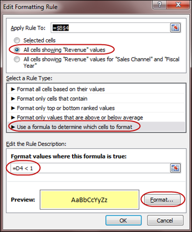
3. In the New Formatting Rule Dialog box:
Apply Rule To: All cells showing “Revenue” values. This is very important…otherwise it’ll only do the one cell which would be difficult to maintain.
Select a Rule Type: Choose the last option, Use a formula to determine which cells to format.
Format values where this formula is true: D4 < 1 (i.e., the Status column is not “green” or “satisfactory”). Make sure there’s no $ signs in this formula. The $ signs make it an absolute reference, and since we want this to apply to all cells showing “Revenue” values, we want it to be a relative reference.
Format: Fill of yellow (or whatever formatting you desire).
And that’s it! You can use this formula-driven method to handle several different conditional formatting options in Excel.
Editing an Existing Rule
To modify the above rule after it’s set up:
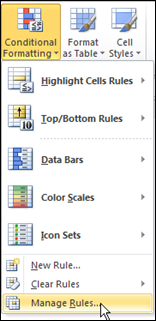
1. Go to Conditional Formatting > Manage Rules.
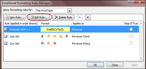
2. Highlight the correct rule and choose Edit Rule. You’ll return to the same window you were working in previously.


